Predict and plot after fitting `arima()` model in R

Question

Just getting acquainted with time series, and using this R-bloggers post as a guide for the following exercise: the futile attempt to predict the future returns in the stock market... Just an exercise in understanding the concept of time series.

The problem is that when I plot the predicted values I get a constant line, which is at odds with the historical data. Here it is, in blue, at the tail end of the stationarized historical Dow Jones daily returns.

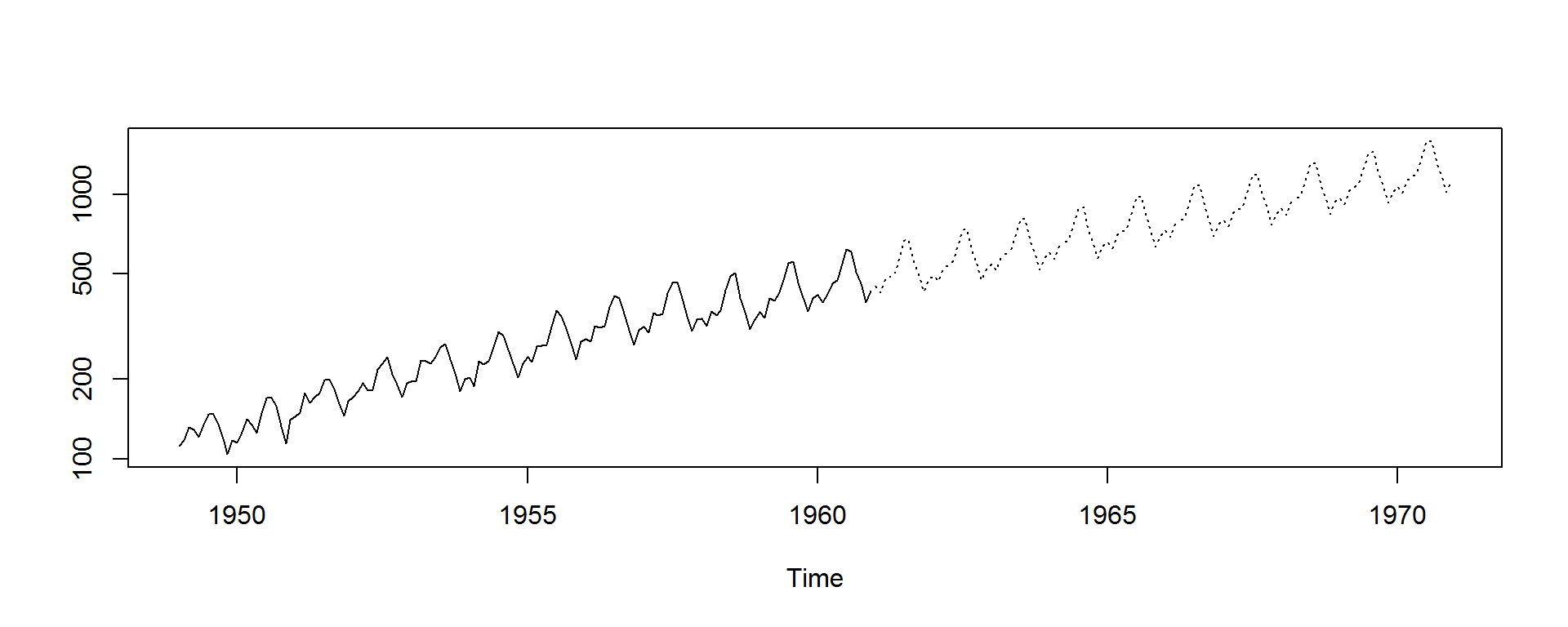
In reality I would like a more "optimistic" visual, or a "re-trended" plot such as the one I got for the predicted number of air travelers:

This is the code:

library(quantmod)
library(tseries)
library(forecast)
getSymbols("^DJI")
d = DJI$DJI.Adjusted
chartSeries(DJI)
adf.test(d) 
dow = 100 * diff(log(d))[-1]
adf.test(dow)
train = dow[1 : (0.9 * length(dow))]
test  = dow[(0.9 * length(dow) + 1):  length(dow)]
fit = arima(train, order = c(2, 0, 2))
predi = predict(fit, n.ahead = (length(dow) - (0.9*length(dow))))$pred
fore  = forecast(fit, h = 500)
plot(fore)

Unfortunately, I get an error if I try the same code use for the air travelers forecast. For example:

fit = arima(log(AirPassengers), c(0, 1, 1), seasonal = list(order = c(0, 1, 1), period = 12))
pred <- predict(fit, n.ahead = 10*12)
ts.plot(AirPassengers,exp(pred$pred), log = "y", lty = c(1,3))

applied to the current problem could possibly (?) go something like this:

fit2 = arima(log(d), c(2, 0, 2))
pred = predict(fit2, n.ahead = 500)
ts.plot(d,exp(pred$pred), log = "y", lty = c(1,3))
Error in .cbind.ts(list(...), .makeNamesTs(...), dframe = dframe, union = TRUE) : non-time series not of the correct length

Answer 1

Making some progress, and the OP is too long as it is.

1. From not working at all to working a bit: Or why I was getting the "non-time series not of the correct length" and other cryptic error messages... Well, without knowing details, it just occurred to me to check what I was trying to cbind.ts: is.ts(d) [1] FALSE Aha! Even if d is an xts object, it is not a time series. So I just had to run as.ts(d). Solved!

2. Unrealistically flat market predictions: Plotting it now as

   fit2 = arima(log(d), c(2, 1, 2)); pred = predict(fit2, n.ahead = 365 * 5) ts.plot(as.ts(d),exp(pred$pred), log = "y", col= c(4,2),lty = c(1,3), main="VIX = 0 Market Conditions", ylim=c(6000,20000))

OK... No prospects for a job at Goldman Sachs with this flat prospect. I need to entice some investors. Let's cook up this snake's oil some more:

3. Getting the flat line going: Let's add up the "seasonality" and we are ready to party like it's 1999:

   fit3 = arima(log(d), c(2, 1, 2), seasonal=list(order = c(0, 1, 1), period=12))

   pred = predict(fit3, n.ahead = 365 * 5) ts.plot(as.ts(d),exp(pred$pred), log = "y", col= c(2,4),lty = c(1,3), main="Investors Prospectus - Maddoff & Co., Inc.")

4. Almost there: I went to John Oliver's page and printed a certificate as an official financial advisor, so I am ready to take your retirement money. In order to do so, I just need to express some healthy uncertainty in this bullish prospect for the next five years. Easy, peasy... fore = forecast(fit2, h = 365 * 5); plot(fore), and voilà...

Oh, no! No way I'm getting any dopes to invest with this reality check... Good thing I didn't quit my daytime job... Wait a second, I messed up entering the model: fore = forecast(fit3, h = 365 * 5) plot(fore):

I'm heading to Staples...