
Reputation: 1
Plotting the velocity vector field in MATLAB
I have a velocity vector u=(ux,uy,uz) which I want to analyse in a mesh grid (see code below). I used the quiver3 function in MATLAB which shows the entire fluid flow in 3-D.
Problem: I wish to see how the velocities change along a 2-D plane only, such that I can visualise how the velocity field changes in x-y plane or z-y plane. How do I do it? I want to plot something similar to this Picture.
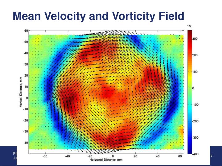
% Parameters
cLx=4;
cLz=2;
a=2*pi/(cLx*pi);
b=pi/2;
g=2*pi/(cLz*pi);
N8=(2*sqrt(2)/sqrt((a*a+g*g)*(4*a*a+4*g*g+pi*pi)));


%Re309
av_val=[0.268359169835888,0.0415737669588199,0.0373076787266736,0.0207721407214892,0.0624519067613835,0.102761062088787,-0.257139476000576,0.0726058071975180,-0.0812934255737902];

% Domain of mesh
% z=0:cLz*pi/20:cLz*pi;
% x=0:cLx*pi/20:cLx*pi;
% y=-1:0.1:1;


[x,y,z]=meshgrid(0:cLx*pi/20:cLx*pi,-1:0.1:1,0:cLz*pi/20:cLz*pi );

% Velocity Equations
ux=av_val(1)*sqrt(2)*sin(pi*y/2) + av_val(2)*(4/sqrt(3))*cos(pi*y/2).*cos(pi*y/2).*cos(g*z) + av_val(6)*4*sqrt(2)/(sqrt(3*(a^2+g*g)))*(-g)*cos(a*x).*cos(pi*y/2).*cos(pi*y/2).*sin(g*z) + av_val(7)*(2*sqrt(2)/(sqrt(a*a+g*g)))*g*sin(a*x).*sin(pi*y/2).*sin(g*z) + av_val(8)*N8*pi*a*sin(a*x).*sin(pi*y/2).*sin(g*z)+ av_val(9)*sqrt(2)*sin(3*pi*y/2);
uy=av_val(3)*(2/(sqrt(4*g*g+pi*pi)))*2*g*cos(pi*y/2).*cos(g*z)+ av_val(8)*N8*2*(a*a+g*g)*cos(a*x).*cos(pi*y/2).*sin(g*z);

uz=av_val(3)*(2/(sqrt(4*g*g+pi*pi)))*pi*sin(pi*y/2).*sin(g*z) + av_val(4)*(4/sqrt(3))*cos(pi*y/2).*cos(pi*y/2).*cos(a*x) + av_val(5)*2*sin(a*x).*sin(pi*y/2) + av_val(6)*(4*sqrt(2)/(sqrt(3*(a*a+g*g))))*a*sin(a*x).*cos(pi*y/2).*cos(pi*y/2).*cos(g*z) + av_val(7)*(2*sqrt(2)/(sqrt(a*a+g*g)))*a*cos(a*x).*sin(pi*y/2).*cos(g*z)- av_val(8)*N8*pi*g*cos(a*x).*sin(pi*y/2).*cos(g*z);


quiver3(x,y,z,ux,uy,uz)
Upvotes: 0
Views: 1386
Answers (1)

Reputation: 118
You need to slice the 3D array by keeping one dimension constant. For example, if you want z-y plane then pick a constant x value. The resulting array would still have three dimensions with a unit length along x. Use the squeeze function to obtain a 2D array. Now you can plot the field in a plane.
Refer to Matlab's help page for curl function, it's a good reference for both computing vorticity and slicing a 3D array.
figure(2)
hold on
x_1d    = 0:cLx*pi/20:cLx*pi;
y_1d    =  -1:0.1:1;
z_1d    = 0:cLz*pi/20:cLz*pi;

slice_x = 11;

uy_yz   = squeeze( uy(slice_x,:,:) );
uz_yz   = squeeze( uz(slice_x,:,:) );

% Compute vorticity - plot as filled contour
vort_yz = curl(y_1d, z_1d, uy_yz, uz_yz);
contourf(y_1d, z_1d, vort_yz)
colorbar()

% Compute 2D-velocity magnitude
% umag_yz = sqrt(uy_yz.^2+uz_yz.^2);
% pcolor(y_1d, z_1d, umag_yz)

% Plot 2D velocity vector
quiver(y_1d, z_1d, uy_yz,uz_yz)
hold off
Upvotes: 1
Related Questions
- `streamline` not plotting this vector field
- How to analyze and visualize a 3D velocity field?
- Quiver - velocity plot Matlab
- How to plot orientation and magnitude of a vector field in Matlab?
- Plotting Vector field of a point charge
- How to plot continuous colored vector field in Matlab?
- Matlab -plot a vector field
- 3d velocity field plotting in matlab
- Vector field in matlab
- Plotting pathlines, streaklines given velocity vector field