How to diagnose what causes OpenModelica transient simulations to run slowly?

Question

I have a transient model with Modelia.Fluid Valves and Dynamic Pipes that is running slowly. I am trying to find strategies and tools for identifying what is causing the slowness. By following the guidance in the Using the Profiler from OMEdit section of the Modelica Performance Analyzer documentation, I am able to see that the non-linear torn systems of equations are taking most of the CPU time which is helpful. However, I would like to learn more about what is causing the simulation to run slowly.

From reading Automatic tracking of stiff calculations in the models for improving simulation performance, it looks like Dymola has a "State variable logging => Which states that dominate error" option that appears to give insight to what part of the model is causing the integration step size to be reduced. I have read through the OpenModelica Compiler Flags and Simulation Flags documentation and have not found a similar option. Does OpenModelica have a similar option? Are there any tools or options within OpenModelica that will help me understand what parts of my model are causing my model to reduce the step size and run slowly or run slowly for other reasons?

If it matters, I am using the DASSL solver and OpenModelica 1.20.0.

Thanks, Michael

2023-03-06 Update in response to Rene Just Nielsen's Feb 17 comment: I suspect that my full system model is too complicated to be helpful so I created a simplified representative example. The full CO2 Deposition (CDep) system is a model of a new system for the removal of carbon dioxide gas from spacecraft cabin air for future NASA missions. This Modeling Performance of the Full Scale CO2 Deposition System paper has a good description of the CDep system and some of our prior modeling work. Since that paper, I have created a model using the Modelica Media ideal gas MixtureGasNasa and Fluid libraries.

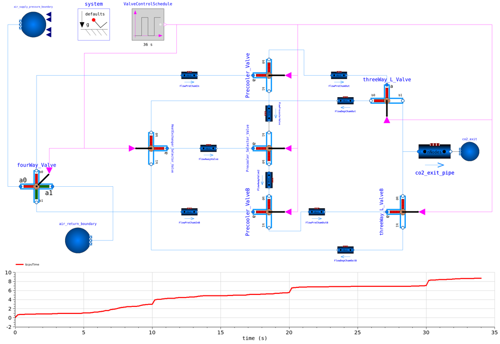
The CDepSystem_valves model in the CDep_Valve_Test_v1p1_20230220.mo library has the same topology as my CDep model. It uses the DynamicPipe model and a three-way valve that I created using the Modelica.Fluid.Valves.ValveDiscreteRamp model. Switching the three-way valve changes flow going into the a-port to flow out of either the b0-port or the b1-port. The default flow path is shown in red. The four-way valve is a simple custom model that connects the pressure supply and the air return boundary to the upper "A" circuit or the lower "B" circuit. The default flow paths through the four-way valve are shown in red and green. The upper vertically oriented pipe and the bottom horizontal pipe do not have flow going through them in the default valve configuration so valve leakage on one end of each of these pipes is used to help stabilize the flow in these pipes. When valves are switched, flow moves through these two pipes and two other pipes stop having flow through them.

The CPU usage plot at the bottom of the image below shows slowness where the valves are switched every 10 seconds. The full CDep system has counter-flow heat exchangers, deposition chambers, and models CO2 and H2O deposition and sublimation. It takes more than an hour of CPU time to model a switching event for the full CDep system. It would be very helpful to understand why modeling the switching events takes so long and figure out how to speed them up. Again, are there any tools or options within OpenModelica that will help me understand what parts of my model are causing my model to reduce the step size and run slowly or run slowly for other reasons?

Answer 1

The model as configured has only a few states. But eventually I assume you will increase nNodes. Then, it will have significantly more continuous time state variables and, because implicit ODE solvers such as Dassl typically scale as O(n^2) to O(n^3) in the number of states n, you can expect slower computing time. You may be able to avoid this by using a pipe model that has plug flow, such as https://github.com/ibpsa/modelica-ibpsa/blob/d4fa56328b4db46bd9e279290ed919285151f588/IBPSA/Fluid/FixedResistances/PlugFlowPipe.mo See https://doi.org/10.1016/j.enconman.2017.08.072 for CPU comparison.

Moreover, each time the model has an event, higher order ODE solvers such as Dassl reinitialize their internal state trajectory approximation by starting with a low order approximation. Sometimes, using a lower order solver, or an explicit solver (if the model is not stiff) can help.

If the physics and dynamics of your problem allows, you may want to approximate the valve opening using a 1st or 2nd order filter, as we often do in the IBPSA library linked above, and replace the ControlSchedule with a differentiable approximation. This way you should be able to avoid the events that cause a solver to restart which can significantly increase computing time.

Answer 2

This answer is not OpenModelica specific, but tested with Dymola 2023x for comparison.

I can open and run your model without any problems and with no errors. Looking over the model, you have applied the staggered grid approach to the valves/pipes, provided initial values and everything looks well thought out!

However, I also get long simulation times when I simulate an hour or a day.

For a two-hour simulation the simulation time can be reduced e.g. by using the default solver setting (DASSL with tolerance set to 1e-4) and by setting the number of output intervals (e.g. 500) rather than storing the variables each 0.2 seconds. In my case this reduces the CPU-time from 107 to is 32.7 seconds.

Unless you need to investigate the fast dynamics from the 10 s switching for hour-long simulations, maybe this could be a part of the solution.