Omitting a Missing x-axis Value in ggplot2 (Convert range to categorical variable)

Question

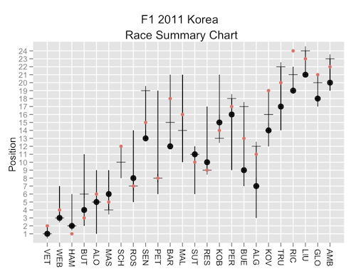
I am using ggplot to generate a chart that summarises a race made up from several laps. There are 24 participants in the race,numbered 1-12, 14-25; I am plotting out a summary measure for each participant using ggplot, but ggplot assumes I want the number range 1-25, rather than categories 1-12, 14-25.

What's the fix for this? Here's the code I am using (the data is sourced from a Google spreadsheet).

sskey='0AmbQbL4Lrd61dHlibmxYa2JyT05Na2pGVUxLWVJYRWc'
library("ggplot2")
require(RCurl)

gsqAPI = function(key,query,gid){ return( read.csv( paste( sep="", 'http://spreadsheets.google.com/tq?', 'tqx=out:csv', '&tq=', curlEscape(query), '&key=', key, '&gid=', curlEscape(gid) ) ) ) }


sin2011racestatsX=gsqAPI(sskey,'select A,B,G',gid='13')
sin2011proximity=gsqAPI(sskey,'select A,B,C',gid='12')

h=sin2011proximity
k=sin2011racestatsX
l=subset(h,lap==1)

ggplot() + 
geom_step(aes(x=h$car, y=h$pos, group=h$car)) + 
scale_x_discrete(limits =c('VET','WEB','HAM','BUT','ALO','MAS','SCH','ROS','SEN','PET','BAR','MAL','','SUT','RES','KOB','PER','BUE','ALG','KOV','TRU','RIC','LIU','GLO','AMB'))+ 
xlab(NULL) + opts(title="F1 2011 Korea \nRace Summary Chart", axis.text.x=theme_text(angle=-90, hjust=0)) + 
geom_point(aes(x=l$car, y=l$pos, pch=3, size=2)) + 
geom_point(aes(x=k$driverNum, y=k$classification,size=2), label='Final') + 
geom_point(aes(x=k$driverNum, y=k$grid, col='red')) + 
ylab("Position")+ 
scale_y_discrete(breaks=1:24,limits=1:24)+ opts(legend.position = "none") 

Answer 1

Expanding on my cryptic comment, try this:

#Convert these to factors with the appropriate labels
# Note that I removed the ''
h$car <- factor(h$car,labels = c('VET','WEB','HAM','BUT','ALO','MAS','SCH','ROS','SEN','PET','BAR','MAL',
                                'SUT','RES','KOB','PER','BUE','ALG','KOV','TRU','RIC','LIU','GLO','AMB'))
k$driverNum <- factor(k$driverNum,labels = c('VET','WEB','HAM','BUT','ALO','MAS','SCH','ROS','SEN','PET','BAR','MAL',
                                'SUT','RES','KOB','PER','BUE','ALG','KOV','TRU','RIC','LIU','GLO','AMB'))
l=subset(h,lap==1)

ggplot() + 
    geom_step(aes(x=h$car, y=h$pos, group=h$car)) + 
    geom_point(aes(x=l$car, y=l$pos, pch=3, size=2)) + 
    geom_point(aes(x=k$driverNum, y=k$classification,size=2), label='Final') + 
    geom_point(aes(x=k$driverNum, y=k$grid, col='red')) + 
    ylab("Position") + 
    scale_y_discrete(breaks=1:24,limits=1:24) + opts(legend.position = "none") + 
    opts(title="F1 2011 Korea \nRace Summary Chart", axis.text.x=theme_text(angle=-90, hjust=0)) + xlab(NULL)

Calling scale_x_discrete is no longer necessary. And stylistically, I prefer putting opts and xlab stuff at the end.

Edit

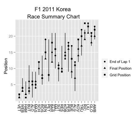
A few notes in response to your comment. Many of your difficulties can be eased by a more streamlined use of ggplot. Your data is in an awkward format:

#Summarise so we can use geom_linerange rather than geom_step
d1 <- ddply(h,.(car),summarise,ymin = min(pos),ymax = max(pos))

#R has a special value for missing data; use it!
k$classification[k$classification == 'null'] <- NA
k$classification <- as.integer(k$classification)

#The other two data sets should be merged and converted to long format    
d2 <- merge(l,k,by.x = "car",by.y = "driverNum")
colnames(d2)[3:5] <- c('End of Lap 1','Final Position','Grid Position')
d2 <- melt(d2,id.vars = 1:2)

#Now the plotting call is much shorter    
ggplot() + 
    geom_linerange(data = d1,aes(x= car, ymin = ymin,ymax = ymax)) + 
    geom_point(data = d2,aes(x= car, y= value,shape = variable),size = 2) + 
    opts(title="F1 2011 Korea \nRace Summary Chart", axis.text.x=theme_text(angle=-90, hjust=0)) + 
    labs(x = NULL, y = "Position", shape = "")

A few notes. You were setting aesthetics to fixed values (size = 2) which should be done outside of aes(). aes() is for mapping variables (i.e. columns) to aesthetics (color, shape, size, etc.). This allows ggplot to intelligently create the legend for you.

Merging the second two data sets and then melting it creates a grouping variable for ggplot to use in the legend. I used the shape aesthetic since a few values overlap; using color may make that hard to spot. In general, ggplot will resist mixing aesthetics into a single legend. If you want to use shape, color and size you'll get three legends.

I prefer setting labels using labs, since you can do them all in one spot. Note that setting the aesthetic label to "" removes the legend title.