XOR neural network backprop

Question

I'm trying to implement basic XOR NN with 1 hidden layer in Python. I'm not understanding the backprop algo specifically, so I've been stuck on getting delta2 and updating the weights...help?

import numpy as np

def sigmoid(x):
    return 1.0 / (1.0 + np.exp(-x))

vec_sigmoid = np.vectorize(sigmoid)

theta1 = np.matrix(np.random.rand(3,3))
theta2 = np.matrix(np.random.rand(3,1))

def fit(x, y, theta1, theta2, learn_rate=.001):
    #forward pass
    layer1 = np.matrix(x, dtype='f')
    layer1 = np.c_[np.ones(1), layer1]
    layer2 = vec_sigmoid(layer1*theta1)
    layer3 = sigmoid(layer2*theta2)

    #backprop
    delta3 = y - layer3
    delta2 = (theta2*delta3) * np.multiply(layer2, 1 - layer2) #??

    #update weights
    theta2 += learn_rate * delta3 #??
    theta1 += learn_rate * delta2 #??

def train(X, Y):
    for _ in range(10000):
        for i in range(4):
            x = X[i]
            y = Y[i]
            fit(x, y, theta1, theta2)


X = [(0,0), (1,0), (0,1), (1,1)]
Y = [0, 1, 1, 0]    
train(X, Y)

Answer 1

OK, so, first, here's the amended code to make yours work.

#! /usr/bin/python

import numpy as np

def sigmoid(x):
    return 1.0 / (1.0 + np.exp(-x))

vec_sigmoid = np.vectorize(sigmoid)

# Binesh - just cleaning it up, so you can easily change the number of hiddens.
# Also, initializing with a heuristic from Yoshua Bengio.
# In many places you were using matrix multiplication and elementwise multiplication
# interchangably... You can't do that.. (So I explicitly changed everything to be
# dot products and multiplies so it's clear.)
input_sz = 2;
hidden_sz = 3;
output_sz = 1;
theta1 = np.matrix(0.5 * np.sqrt(6.0 / (input_sz+hidden_sz)) * (np.random.rand(1+input_sz,hidden_sz)-0.5))
theta2 = np.matrix(0.5 * np.sqrt(6.0 / (hidden_sz+output_sz)) * (np.random.rand(1+hidden_sz,output_sz)-0.5))

def fit(x, y, theta1, theta2, learn_rate=.1):
    #forward pass
    layer1 = np.matrix(x, dtype='f')
    layer1 = np.c_[np.ones(1), layer1]
    # Binesh - for layer2 we need to add a bias term.
    layer2 = np.c_[np.ones(1), vec_sigmoid(layer1.dot(theta1))]
    layer3 = sigmoid(layer2.dot(theta2))

    #backprop
    delta3 = y - layer3
    # Binesh - In reality, this is the _negative_ derivative of the cross entropy function
    # wrt the _input_ to the final sigmoid function.

    delta2 = np.multiply(delta3.dot(theta2.T), np.multiply(layer2, (1-layer2)))
    # Binesh - We actually don't use the delta for the bias term. (What would be the point?
    # it has no inputs. Hence the line below.
    delta2 = delta2[:,1:]

    # But, delta's are just derivatives wrt the inputs to the sigmoid.
    # We don't add those to theta directly. We have to multiply these by
    # the preceding layer to get the theta2d's and theta1d's
    theta2d = np.dot(layer2.T, delta3)
    theta1d = np.dot(layer1.T, delta2)

    #update weights
    # Binesh - here you had delta3 and delta2... Those are not the
    # the derivatives wrt the theta's, they are the derivatives wrt
    # the inputs to the sigmoids.. (As I mention above)
    theta2 += learn_rate * theta2d #??
    theta1 += learn_rate * theta1d #??

def train(X, Y):
    for _ in range(10000):
        for i in range(4):
            x = X[i]
            y = Y[i]
            fit(x, y, theta1, theta2)


# Binesh - Here's a little test function to see that it actually works
def test(X):
    for i in range(4):
        layer1 = np.matrix(X[i],dtype='f')
        layer1 = np.c_[np.ones(1), layer1]
        layer2 = np.c_[np.ones(1), vec_sigmoid(layer1.dot(theta1))]
        layer3 = sigmoid(layer2.dot(theta2))
        print "%d xor %d = %.7f" % (layer1[0,1], layer1[0,2], layer3[0,0])

X = [(0,0), (1,0), (0,1), (1,1)]
Y = [0, 1, 1, 0]    
train(X, Y)

# Binesh - Alright, let's see!
test(X)

And, now for some explanation. Forgive the crude drawing. It was just easier to take a picture than draw something in gimp.

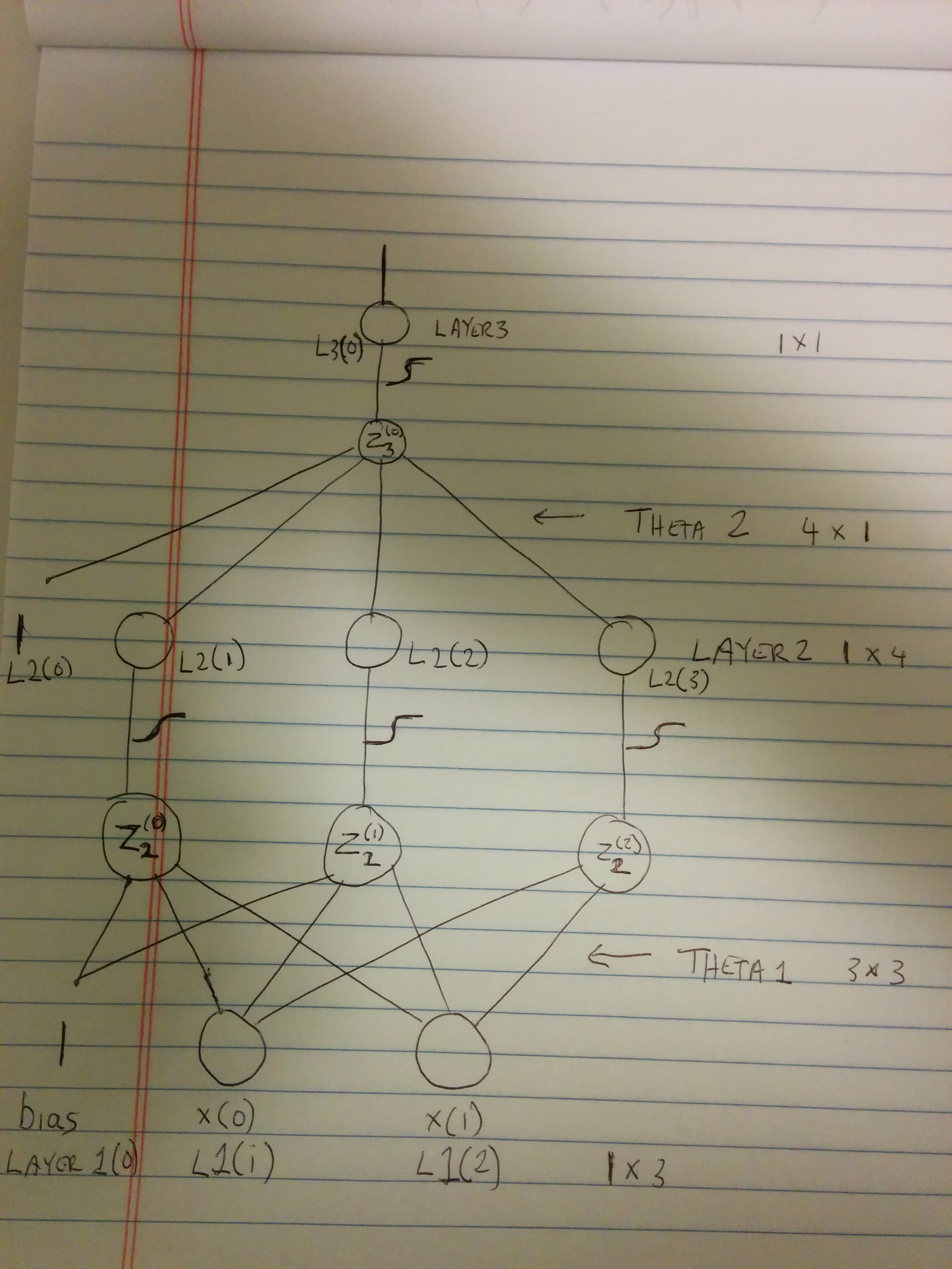
_{(source: binesh at cablemodem.hex21.com)}

So. First, we have our error function. We'll call this CE (for Cross Entropy. I'll try to use your variables where possible, tho, I'm going to use L1, L2 and L3 instead of layer1, layer2 and layer3. sigh (I don't know how to do latex here. It seems to work on the statistics stack exchange. weird.)

CE = -(Y log(L3) + (1-Y) log(1-L3))

We need to take the derivative of this wrt L3, so that we can see how we can move L3 so as to reduce this value.

dCE/dL3 = -((Y/L3) - (1-Y)/(1-L3))
        = -((Y(1-L3) - (1-Y)L3) / (L3(1-L3)))
        = -(((Y-Y*L3) - (L3-Y*L3)) / (L3(1-L3)))
        = -((Y-Y3*L3 + Y3*L3 - L3) / (L3(1-L3)))
        = -((Y-L3) / (L3(1-L3)))
        = ((L3-Y) / (L3(1-L3)))

Great, but, actually, we can't just alter L3 as we see fit. L3 is a function of Z3 (See my picture).

L3      = sigmoid(Z3)
dL3/dZ3 = L3(1-L3)

I'm not deriving this here, (the derivative of the sigmoid) but, it's actually not that hard to prove).

But, anyway, that's the derivative of L3 wrt Z3, but we want the derivative of CE wrt Z3.

dCE/dZ3 = (dCE/dL3) * (dL3/dZ3)
        = ((L3-Y)/(L3(1-L3)) * (L3(1-L3)) # Hey, look at that. The denominator gets cancelled out and
        = (L3-Y) # This is why in my comments I was saying what you are computing is the _negative_ derivative.

We call the derivatives wrt Z's "deltas". So, in your code, this corresponds to delta3.

Great, but we can't just change Z3 as we like either. We need to compute it's derivative wrt L2.

But this is more complicated.

Z3 = theta2(0) + theta2(1) * L2(1) + theta2(2) * L2(2) + theta2(3) * L2(3)

So, we need to take partial derivatives wrt. L2(1), L2(2) and L2(3)

dZ3/dL2(1) = theta2(1)
dZ3/dL2(2) = theta2(2)
dZ3/dL2(3) = theta2(3)

Notice that the bias would effectively be

dZ3/dBias  = theta2(0)

but the bias never changes, it's always 1, so we can safely ignore it. But, our layer2 includes the bias, so we'll keep it for now.

But, again, we want the derivative wrt Z2(0), Z2(1), Z2(2) (Looks like I drew that badly, unfortunately. Look at the graph, it'll be clearer with it, I think.)

dL2(1)/dZ2(0) = L2(1) * (1-L2(1))
dL2(2)/dZ2(1) = L2(2) * (1-L2(2))
dL2(3)/dZ2(2) = L2(3) * (1-L2(3))

What now is dCE/dZ2(0..2)

dCE/dZ2(0) = dCE/dZ3 * dZ3/dL2(1) * dL2(1)/dZ2(0)
           = (L3-Y)  * theta2(1)  * L2(1) * (1-L2(1))

dCE/dZ2(1) = dCE/dZ3 * dZ3/dL2(2) * dL2(2)/dZ2(1)
           = (L3-Y)  * theta2(2)  * L2(2) * (1-L2(2))

dCE/dZ2(2) = dCE/dZ3 * dZ3/dL2(3) * dL2(3)/dZ2(2)
           = (L3-Y)  * theta2(3)  * L2(3) * (1-L2(3))

But, really we can express this as (delta3 * Transpose[theta2]) elemenwise multiplied by (L2 * (1-L2)) (where L2 is the vector)

These are our delta2 layer. I remove the first entry of it, because as I mention above, it corresponds to the delta of the bias (what I label L2(0) on my graph.)

So. Now, we have derivatives wrt our Z's, but, really, what we can modify are only our thetas.

Z3 = theta2(0) + theta2(1) * L2(1) + theta2(2) * L2(2) + theta2(3) * L2(3)
dZ3/dtheta2(0) = 1
dZ3/dtheta2(1) = L2(1)
dZ3/dtheta2(2) = L2(2)
dZ3/dtheta2(3) = L2(3)

Once again tho, we want dCE/dtheta2(0) tho, so that becomes

dCE/dtheta2(0) = dCE/dZ3 * dZ3/dtheta2(0)
               = (L3-Y) * 1
dCE/dtheta2(1) = dCE/dZ3 * dZ3/dtheta2(1)
               = (L3-Y) * L2(1)
dCE/dtheta2(2) = dCE/dZ3 * dZ3/dtheta2(2)
               = (L3-Y) * L2(2)
dCE/dtheta2(3) = dCE/dZ3 * dZ3/dtheta2(3)
               = (L3-Y) * L2(3)

Well, this is just np.dot(layer2.T, delta3), and that's what I have in theta2d

And, similarly: Z2(0) = theta1(0,0) + theta1(1,0) * L1(1) + theta1(2,0) * L1(2) dZ2(0)/dtheta1(0,0) = 1 dZ2(0)/dtheta1(1,0) = L1(1) dZ2(0)/dtheta1(2,0) = L1(2)

Z2(1) = theta1(0,1) + theta1(1,1) * L1(1) + theta1(2,1) * L1(2)
dZ2(1)/dtheta1(0,1) = 1
dZ2(1)/dtheta1(1,1) = L1(1)
dZ2(1)/dtheta1(2,1) = L1(2)

Z2(2) = theta1(0,2) + theta1(1,2) * L1(1) + theta1(2,2) * L1(2)
dZ2(2)/dtheta1(0,2) = 1
dZ2(2)/dtheta1(1,2) = L1(1)
dZ2(2)/dtheta1(2,2) = L1(2)

And, we'd have to multiply by dCE/dZ2(0), dCE/dZ2(1) and dCE/dZ2(2) (for each of the three groups up there. But, if you think about that, that then just becomes np.dot(layer1.T, delta2), and that's what I have in theta1d.

Now, because you did Y-L3 in your code, you're adding to theta1 and theta2... But, here's the reasoning. What we just computed above is the derivative of CE wrt the weights. So, that means, increasing the weights by will increase the CE. But, we really want to decrease the CE.. So, we subtract (normally). But, because in your code, you're computing the negative derivative, it is right that you add.

Does that make sense?